Exercises 7.5 Chapter Test
1.
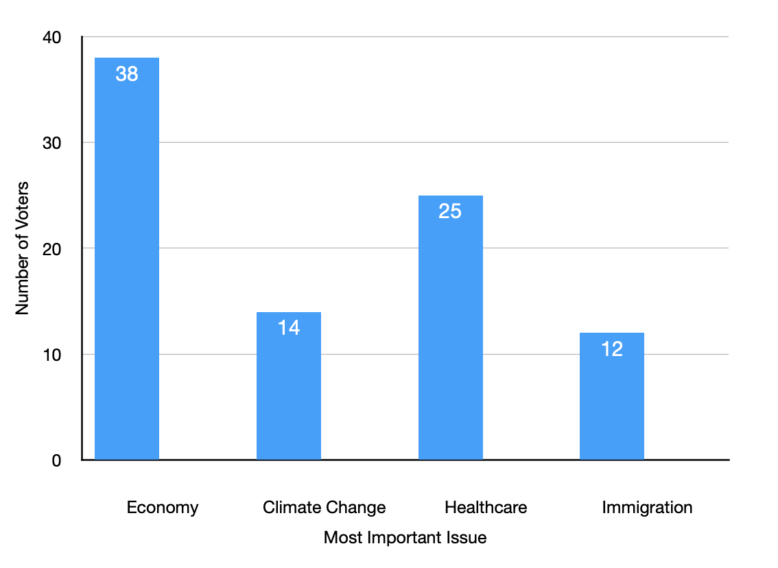
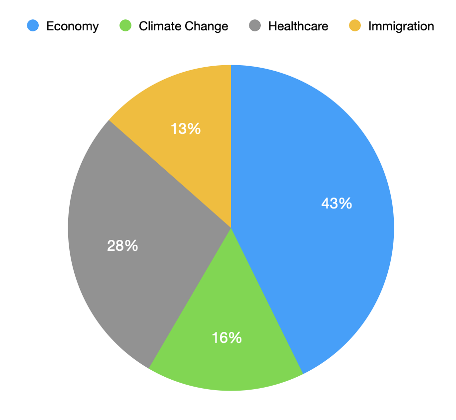
A group of voters was surveyed about the issues that are most important to them. The results are summarized in the table.
Number of Respondants
Most Important Issue
38
Economy
14
Climate Change
25
Healthcare
12
Immigration
How many people were surveyed?
Create a bar graph to display this data.
Create a pie chart to display this data.
89
2.
Scores on a test are given below. Organize this data into class intervals with a width of 5, starting at 30. Create a histogram for the data.
48, 53, 32, 41, 46, 33, 42, 51, 36, 37, 47, 39, 54, 33, 48, 40, 36, 35, 49, 52, 39, 44
Greater than or equal to
Less than
Frequency
30
35
3
35
40
6
40
45
4
45
50
5
50
55
4

3.
For the dataset:
Find mean, median, and mode.
Give the 5-number summary.
Find sample standard deviation.
\(\mu = 6.09\text{,}\) \(M = 8\text{,}\) mode \(=8\)
Min = 1, Q1 = 3, Median = 8, Q3 = 8, Max = 9
2.98
-
The mean is the sum of the values, divided by the number of values:
\begin{equation*} \mu = \frac{8+4+8+9+8+7+3+2+1+9+8}{11} = \frac{67}{11}=6.09 \end{equation*} -
The five-number summary consists of the max, min, median, 1st quartile and 3rd quartile.
Maximum = 9, Minimum = 1, Median = 8.
To find the 1st quartile, \(L = 0.25(11) = 2.75\text{.}\) We round up and look at the 3rd value. \(Q_1 = 3\text{.}\)
To find the 3rd quartile, \(L = 0.75(11) = 8.25\text{.}\) We round up and look at the 9th value. \(Q_3 = 8\text{.}\)
-
We will added up squared deviations, divide by 10 (\(n - 1\)) and then take the square root of the result.
Table 7.5.4. Frequency \(x\) \(x - \mu\) \((x - \mu)^2\) 1 1 \(1 - 6.09 = -5.09\) \((-5.09)^2=25.9081\) 1 2 \(2 - 6.09 = -4.09\) \((-4.09)^2=16.7281\) 1 3 \(3 - 6.09 = -3.09\) \((-3.09)^2=9.5481\) 1 4 \(4 - 6.09 = -2.09\) \((-2.09)^2=4.3681\) 1 7 \(7 - 6.09 = 0.91\) \((0.91)^2=0.8281\) 4 8 \(8 - 6.09 = 1.91\) \((1.91)^2=3.6481\) 2 9 \(9 - 6.09 = 2.91\) \((2.91)^2=8.4681\) The sum of the squared deviations is:
\begin{equation*} 25.9081+16.7281+9.5481+4.3681+0.8281+4\cdot 3.6481+2 \cdot 8.4681=88.9091 \end{equation*}Divide by \(n-1=10\) and take the square root:
\begin{equation*} \sqrt{\frac{88.9091}{10}}=2.98 \end{equation*}
4.
The table below gives the heights (in inches) of a women’s basketball team.
Height
Frequency
64
1
65
2
67
3
68
6
69
4
70
5
72
1
73
1
Find the mean height.
Find the median height.
Find the first and third quartile.
Find the population standard deviation.
Create a box-and-whiskers plot.
68.4 inches
68 inches
\(\displaystyle Q_1 = 67, Q_3 = 70\)
2.06 inches
See solution.
There are \(n = 1+2+3+6+4+5+1+1=23\)values.
\begin{equation*} \mu = \frac{1\cdot 64 + 2\cdot 65 + 3 \cdot 67 + 6 \cdot 68 + 4 \cdot 69 + 5 \cdot 70 + 1 \cdot 72 + 1 \cdot 73}{23} \end{equation*}\begin{equation*} \mu = \frac{1574}{23}=68.4 \end{equation*}-
There are \(n = 23\) values. To find the median, \(L = 0.5(23) = 11.5\text{.}\) Round up and look at the 12th value.
Table 7.5.6. Height Frequency Values 64 1 1 65 2 2 - 3 67 3 4 - 6 68 6 7 - 12 69 4 13 - 16 70 5 17 - 21 72 1 22 73 1 23 The 12th value is 68. \(M = 68\text{.}\)
-
To find the 1st quartile, \(L = 0.25(23)=5.75\text{.}\) Round up and look at the 6th value. \(Q_1 = 67\text{.}\)
To find the 3rd quartile, \(L = 0.75(23) = 17.25\text{.}\) Round up and look at the 18th value. \(Q_3 = 70\text{.}\)
-
To find the population standard deviation, add up squared deviations from the mean, divide by the number values in the dataset, and take the square root.
Table 7.5.7. Frequency \(x\) \(x - \mu\) \((x-\mu)^2\) 1 \(64\) \(64 - 68.4 = -4.4\) \((-4.4)^2 = 19.36\) 2 \(65\) \(65 - 68.4 = -3.4\) \((-3.4)^2 = 11.56\) 3 \(67\) \(67 - 68.4 = -1.4\) \((-1.4)^2 = 1.96\) 6 \(68\) \(68 - 68.4 = -0.4\) \((-0.4)^2 = 0.16\) 4 \(69\) \(69 - 68.4 = 0.6\) \((0.6)^2 = 0.36\) 5 \(70\) \(70 - 68.4 = 1.6\) \((1.6)^2 = 2.56\) 1 \(72\) \(72 - 68.4 = 3.6\) \((3.6)^2 = 12.96\) 1 \(73\) \(73 - 68.4 = 4.6\) \((4.6)^2 = 21.16\) Add up the squared deviations, by multiplyig them by their frequencies:
\begin{equation*} 1 \cdot 19.36+2\cdot 11.56+3 \cdot 1.96 + 6\cdot 0.16 + 4\cdot 0.36+5\cdot 2.56 + 1\cdot 12.96 + 1 \cdot 21.16 = 97.68 \end{equation*}Then divide by \(n = 23\) and take the square root:
\begin{equation*} \sqrt{\frac{97.68}{23}}=2.06 \end{equation*} - The box will extend from \(Q_1 = 67\) to \(Q_3 = 70\) with a line drawn at the median, \(M = 68\text{.}\) The whiskers extend from the minimum value of \(64\) to the maximum value of \(73\text{.}\)

Figure 7.5.8. Image Credit: RRCC
5.
The box plots below show the ages of both men and women Olympic gymnasts. Use the box plots to answer the following questions.

What is the median age of a female Olympic gymnast?
25% of the female gymnasts are ___ or older.
____ % of the male gymnasts are 23 or younger.
Which gender has a larger range in ages of athletes?
17
16
50%
Male gymnast ages have a larger range.
6.
The mean price of a dozen eggs is $2.19 with a standard deviation of $0.09. The mean price of a pound of chicken is $5.89 with a standard deviation of $0.15. Which item had more variability in prices? Explain.
The coefficient of variation for the eggs is:
The coefficient of varation for the chicken is:
Since the coefficient of varation is larger for the eggs, there is more variability in egg prices than chicken.